Wave Machine: Determining the sea conditions for cargo ships
Project Description
This project aims to extract the sea conditions that a cargo ship is experiencing using time series data from 4 different draft sensors installed in the ship. The draft sensors provide water depth information at each position of the ship where the corresponding sensor is installed. Currently the sea conditions are daily reported by the captain, and the goal of this project is to build a model to automate the captain's report on the sea conditions using the draft sensor data.
This information on the sea conditions would eventually allow a maritime consulting company to make suggestions for how the ship can burn less fuel.
1. What are the sea conditions?
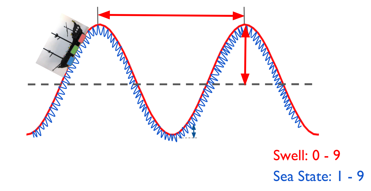
The sea conditions are determined by two parameters, Swell and Sea State. Swell is given by large wave structure (imagine there's a hurricane far away and a big wave propagates to where the ship is). Sea state is about the choppiness of the water surface where the ship is. For example, local wind can generate ripples at the sea surface around the ship and it can change the Sea State. Fig. 1 shows a cartoon describing the Swell and Sea State shown in red in blue, respectively. A Swell wave roughly consists of Sea State waves. Swell is described by both length (red horizontal arrow) and height (red vertical arrow) of the wave, while Sea State is determined only by the height (blue vertical arrow).
The captain on the ship reports the sea conditions with daily the codes on both Swell and Sea State. For example, the captain could report the Swell and Sea State as "04 MODERATE SWELL Height, AVERAGE Length" and "03 SLIGHT Sea State Height".
Using the data from the draft sensors, located at forward, middle, and aft (shown as red, green, and blue boxes in Fig 1.), we want to reconstruct the wave structure for both Swell and Sea State. By correlating the wave information obtained from the draft sensors to the captain's daily report at a given time, we wish to build a model to determine the sea state with the Swell and Sea State codes.
2. Data Challenges and Solutions
2.1. Challenges
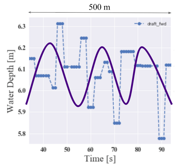
The first thing to verify is whether we can see a wave structure from the draft sensor readings. However, as shown in Fig. 2, it is not possible to see any wave-like structure from the draft sensors. We need to think of other features which reflect the sea conditions rather than try to fully reconstruct the wave.
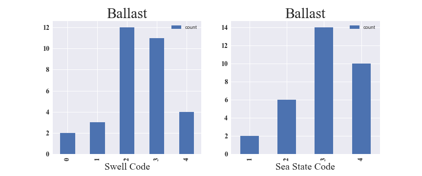
Another challenge is the very small number of captain's daily reports. The captain's daily log is available from April 14, 2017, and only two months of data has been accumulated as of Jun 25, 2017. In addition, the dataset has to be split into two cases depending on the cargo conditions. When a cargo ship is not loaded with cargo and in the "ballast" state, the ship's weight is about two times lighter and the draft sensors yield smaller water depth values. Also, in the ballast state, the ship is tilted (cargo is loaded at the aft of the ship) and the forward sensor is always reading a higher value than the aft sensor. In total, we have 32 and 21 captain's log available for the ballast and laden (the ship is fully loaded with cargo) states, respectively. Even if we choose the ballast state, these 32 data points are spread into 5 (4) categories for Swell (Sea State) codes as shown in Fig 3. We do not have any data avaialble with more extreme conditions with higher code values.
2.2. Solutions
To tackle the challenge that the draft sensor did not exhibit wave-like structure, I designed a feature which could be sensitive to sea conditions. The most natural guess was that when the sea condition is extreme, the ship will be shakier and the draft sensor value itself will fluctuate more. Indeed the data supported this guess. Also, given that the ship is tiled in the ballast state, the difference between two sensors, especially between forward and aft sensors, would be most sensitive to any fluctuation of the ship. Therefore, I came up with a feature defined as the standard deviation of the difference between forward and aft sensors, normalized by the mean of the differnece. To obtain the standard deviation and the mean, I merged the samples within 150 seconds. I assumed that the sea condition stayed the same within two hours (which gives me 48 data points) and took the mean of the distribution as the feature.
The second thing I did was reframe the problem as a binomial logistic regression problem (sea is calm or moderate) rather than a multinomial logistic regression problem (swell codes ranges from 0 to 4). Some of the categories have only one or two entries and 32 data points are not enough to perform multinomial logistic regression.
Lastly, I decided to use probablistic programming using Bayesian inference for this specific problem. Rather than divide the datasets into training and test datasets, using all the data to build the model and verify it with Monte Carlo simultion based on the posterior seemed to be a better approach. In addition, this method provides not only the probability that the sea is moderate but also the associated uncertainty of the probability. With limited statistics, I think it is more important to provide proper uncertainty of the classification.
3. Model
3.1 The sea is calm or moderate?
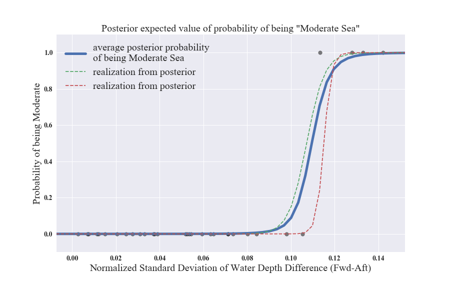
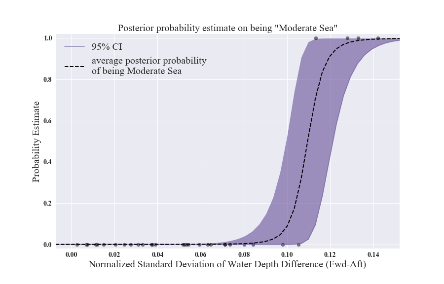
Once we reframe the problem as a binomial logistic regression problem, we can describe the probability of the sea being moderate as a function of the feature described in Section 2.2. I used the PyMC3 package and used the Metropolis-Hasting algorithm to obtain the posterior distribution of the two coefficients in the logisitc function. Fig 4. shows the data points (shown as gray dots) along with the average posterior (shown as a blue line), and two specific cases of obtained posterior selections after burning a million samples. The blue line is the deliverable of this project!
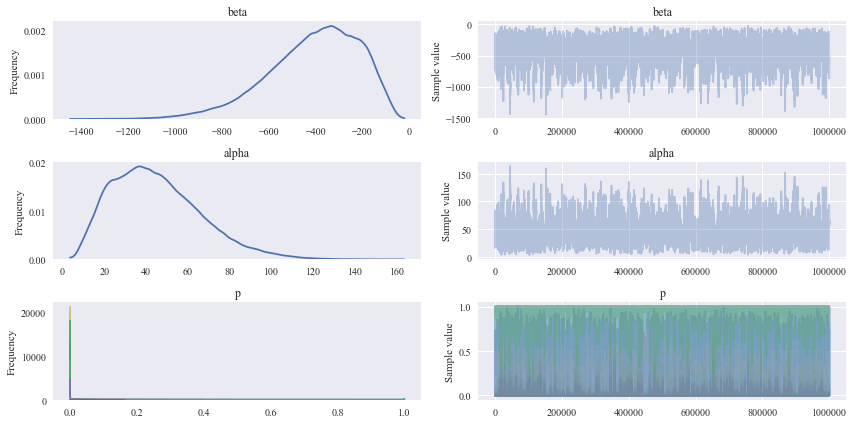
3.2 How good was the Markov Chain Monte Carlo sampling?
To obtain reasonable posterior distributions, I have generated 1000000 samples, burned 150000 of them, and used a thin of 10. As shown in Fig. 5, the optimization of the posterior obtainment was successful (no discrete structure in both posterior distributions as well as trace evolution.)
3.3 What is the uncertainty on the probability of determining the sea conditions?
Since we have the posterior distributions on the model, we can also obtain the associate uncertainty on the probability of the sea being moderate. Fig 6 shows 95% Confidence Interval (C.I.) of the probability with purple band. C.I. means 95% of the posterior distribution lies within the band. As shown in the figure, we can be certain that the sea is calm where the feature value is below 0.06, as well as above 0.14 the sea is moderate. However, at the value around 0.11, the C.I. provides wildy varying values from ~ 0.02 to 1, while the probability of being in the moderate state is 0.8. Basically we are not able to robustly classify the sea condition as calm or moderate when the observed feature value lies between 0.10 and 0.12.
3.4 How good is the model?
To verify that the model is good, we can generate an aritificial dataset using the info obtained from the posterior and make a comparison with the observations we have. The idea here is that if the simulated data is not similar to the observation statistically, our model does not represent the data correctly. We can think that the observation is a specific case of the posterior distributions and see how probable it is statistically.
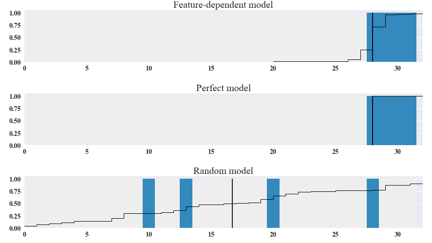
Fig 7. shows three models to get an idea about how good our model (top) is. For each model, we calculate the proportion of times the posterior simulation is a value of 1 for a particular feature value. It gives the posterior probability of the sea being moderate at each data point. If we sort them by the posterior probability, we obtain the plot where the occurence of the sea being moderate is indicated as a blue box and the probability of the sea being moderate is shown as a horizontal black line, while the vertical line shows the threshold separating calm and moderate conditions. This separation plot also allows the user to see how the total number of events predicted by the model compares to the actual number of events in the data.
The perfect model would predict the sea being moderate with probability 1 for the occurence of the sea being moderate and 0 for the sea being calm as shown in the middle plot of Fig 7. For random probability distribution for the sea being moderate, it will just randomly occur at any probability order. As we can see in Fig 7, the feature-dependent model yields the occurence of the sea being moderate correctly right to the separation line.
3.5 What could be improved?
There are several things that could be improved for the current analysis but the main requirement is having more data in the Captain's log. We could consider increasing the corresponding data points for each captain's log by having multiple values for the feature mentioned in Sec. 2.2. by enlarging the time window and separating different time slots (e.g., instead of looking at 1 feature value obtained within 2 hours, we could obtain 3 values with a 1 hour separation in 3 hours). However, given that we are already using the mean behavior of the feature within a certain time window, it would not change the probability distribution function significantly with the current Bayesian approach. It might be more suitiable for the other approaches such as random forest and could be interesting to compare the results.
Once we have more data we could go back and try to perform multinomial logistic regression. In addition to multinomial logistic regression, we could consider ordinal regression too.
Lastly, given that we did not observe any wave structure with the existing sensors, it could be worth taking data with other types of sensors. One of the limitations of the current sensor data comes from the fact that the ship dimension is often larger than the Swell wave length and it would not be easy to see the smaller structure. It might be more useful to have a small vessel instrumented with the sensors which could see the wave structure for both Swell and Sea State. Also, we can think of completely different types of sensors such as gyroscopes or image processing of a sattelite image of the sea around the ship.
4. Business Applications
The model used for this analysis can be applied to any problem with small labeled data for classification. For example, it can be used to determine car failure rate using the sensor reading on the car. Another use could be to determine health insurance plans for rare diseases. Startup company marketing advice with limited initial statistics could be an application too.
Acknowledgement
This project was done in collobration with Nautilus Labs, a maritime consulting company. Nautilus Labs aims to make data-driven advices on the ship operation to reduce not only the cost but also the air pollution through less fuel burning, which has significant impact on both global economy and environment. Details on Nautilus Labs can be found here. I would like to thank Brian and Anthony for providing the data and knoweldge of the ship, and Daniel for the mentorship.